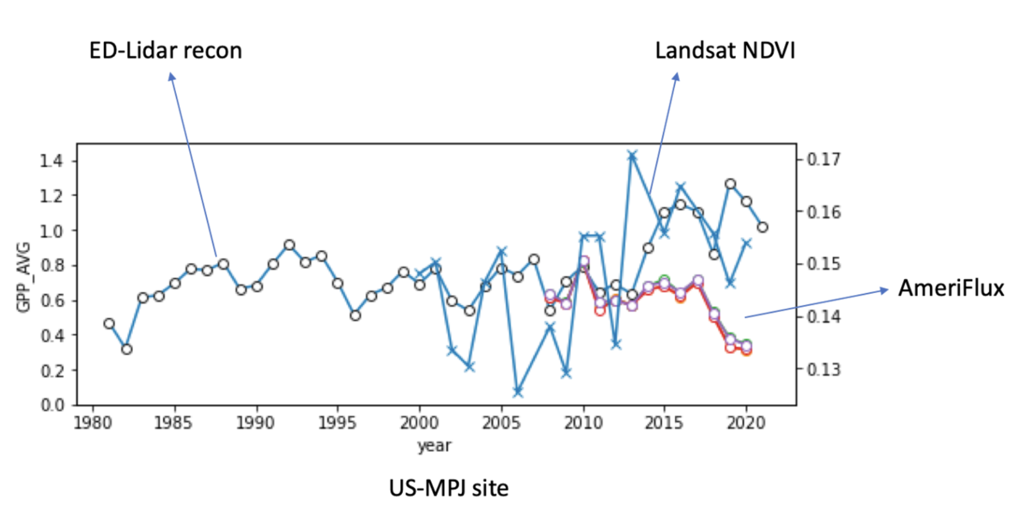
The sharp divergence between ED-Lidar reconstructions, Landsat NDVI, and AmeriFlux GPP observations (see figure) around 2010–2020 sparked this investigation. While historical reconstructions suggest stable or even rising productivity, both satellite vegetation indices (NDVI) and flux tower data show a clear decline in GPP at the US-MPJ site during this period.
This discrepancy raised a key question: Is this ecosystem experiencing large-scale tree mortality that is not being captured by traditional models?
To answer this, I developed an image-based approach to directly detect vegetation loss and tree death from aerial imagery, aiming to complement and explain these broader ecosystem signals. This report is a log of various initial approaches which were not pursued further due to inconclusive results. The final log throws light on the current approach being pursued due to its promising nature. The later research reports help to track tree mortality and its various real-world applications for NASA CMS etc.
DeepForest Approach
I focus on how to reliably detect tree mortality across time using aerial imagery? Can pretrained object detection models, like DeepForest, give us useful indicators of tree health or death?
DeepForest is a SOTA model trained on RGB imagery to detect individual tree crowns. It outputs bounding boxes around tree-like objects, which initially seemed promising for analyzing:
- Tree count changes over time
- Tree canopy shrinkage
- Mortality via absence or degradation of detected crowns
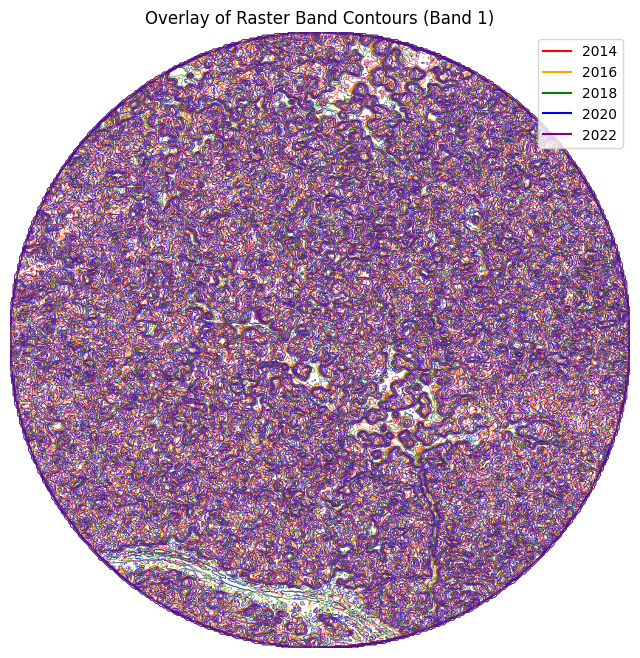
I use a pretrained model to quickly extract structured detections and use bounding box count or size as a proxy for forest density. This would be the first step towards detecting tree loss trends over time without training from scratch. Iused NAIP imagery from 2014-2022 split into 512x512 tiles. One interesting thing to note was the resolution change from 1.0m to 0.6m during the transition year of 2018.
from deepforest import main
model = main.deepforest()
model.use_release()
boxes = model.predict_image(path="naip_tile.png", return_plot=True)
Sample Outputs
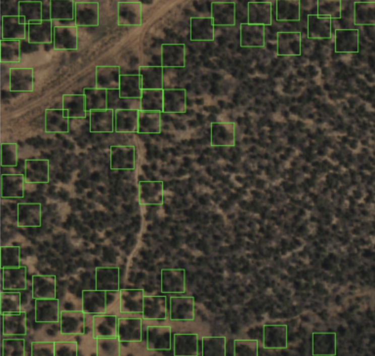
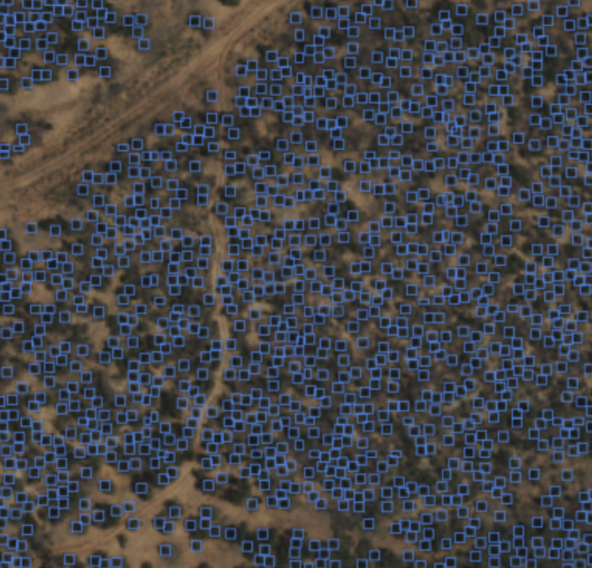
While promising, the spatial resolution mismatch meant Icould not perform any temporal analysis. To add, DeeForest was trained on ~0.1m resolution which led to noisy predictoins due to the coarse nature of our NAIP tiles (1.0m/0.6m). Another key issue was that bounding boxes around trees did not necessarily translate to tree area, invalidating any use of true detection – which varied erratically due to visual artifacts.
In summary, visual interpretability, spatial precision, and temporal consistency were all poor leading to exploring alternative approaches.
Patch-Based Classification
I needed a strategy focused on semantic labeling (LIVE / DEAD / BARE), not detection. This led to the 5x5 patch-based classification approach. The goal was to label small regions of aerial imagery based on ecological intuition, using spatial patches instead of pixel-level or bounding box classification.
Each 512×512 tile was divided into a 5×5 grid (i.e. ~25×25 pixel patches). Each patch was visually labeled based on dominant appearance: LIVE, DEAD, or BARE. The thought process was this was smoother than pixel classification yet easier than labeling full tiles while providing enough context for human labeling (e.g., sparse vs dense canopy).
I recorded each tile into patches with relevant metadata. A sample record would read as r329_c58_y2020.png, 329, 58, 2020, , possibly BARE or DEAD. Labels were then assigned via manual inspection across year with texture, color and shape being taken into account. I then make a simple RandomForest model (baseline) with RGB stats as our core features.
Sample Outputs

This was a promising direction but had drawbacks. For instance, I encountered labeling conflicts with mixed-content patches (e.g., half LIVE, half DEAD) making it very subjective. The spectral and spatial inconsistencies were more complex at the patch level with the model failing to generalize across years.
| Metric | Result |
|---|---|
| In-year Accuracy | ~65–70% |
| Cross-year Generalization | Failed (<50%) |
| Label Noise | High |
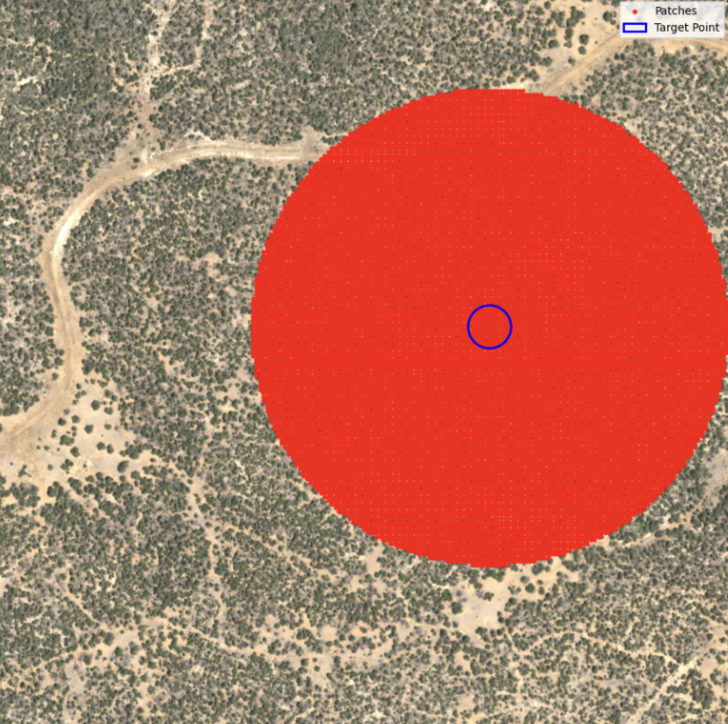
Single Pixel Temporal Classification
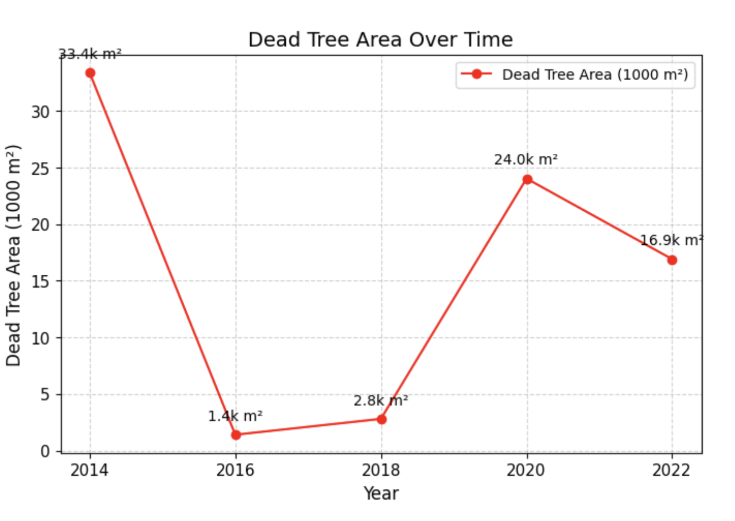
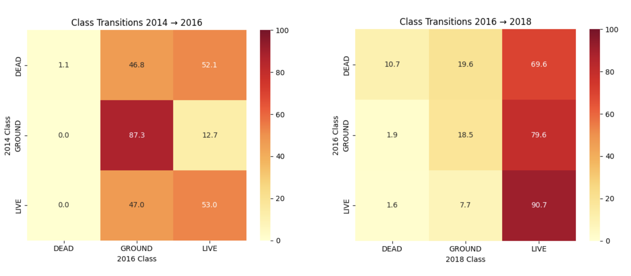
To resolve both spectral and spatial instability, I transitioned to pixel-level temporal modeling — tracking individual pixels across all years and use their temporal NDVI trajectories to classify them into ecological categories (LIVE, DEAD, BARE). With this approach, I now gain control over exact spatial location and can detect transitions across years. I also included NDVI data as part of the labeling strategy.
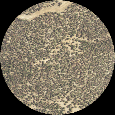
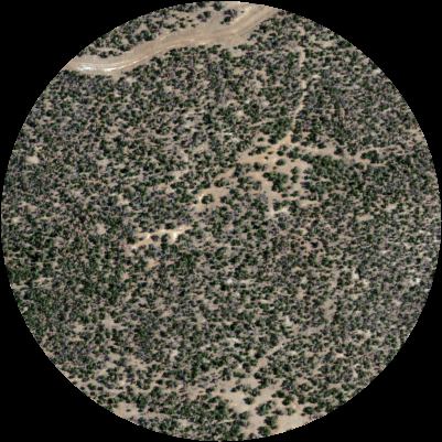
Sample Outputs
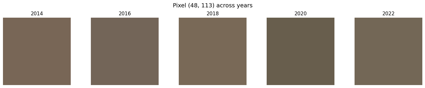
The benefits of this approach were multifold. Now, I can solve for spectral inconsistencies and apply spatial registration corrections to study transitions with high accuracy.
| Metric | Result |
|---|---|
| Temporal NDVI consistency | Strong |
| Human label quality | High confidence |
| Class balance | Still tuning |
| Next step | Expand labeled samples & train temporal classifier |
Refer here for all research reports.