Motivation
Accurate analysis of temporal vegetation transitions—such as LIVE → DEAD or DEAD → BARE—requires reliable alignment of pixels across years. Even after spatial preprocessing like warping and histogram matching, small-scale spatial drift can occur, especially in high-resolution NAIP imagery.
This poses a significant problem for longitudinal classification. If the same (row, col) location in one year corresponds to a slightly shifted feature in another (e.g., shadow, soil), observed changes may reflect misalignment rather than ecological dynamics.
To rigorously evaluate class transitions and develop robust temporal models, we must quantify and control for this drift.
Identifying a Fixed Reference Point
To ground the analysis, we manually located a visually bright, highly consistent white patch—most likely a man-made structure or tower—within the 2014 NAIP image. This was done using RGB previews of the matched_buffer_{year}.tif files in QGIS.
We then traced this patch across earlier years and visually validated its shifted position in 2016 and 2018. The corresponding row/column locations are:
| Year | Row | Col |
|---|---|---|
| 2014 | 119 | 224 |
| 2016 | 121 | 224 |
| 2018 | 118 | 224 |
No precise match could be confirmed for 2020 and 2022, likely due to changes in lighting conditions or NDVI spectral compression in post-processing.
Understanding Spatial Drift
We define three conceptual degrees of spatial drift:
-
Level 1: Linear Shift
Straightforward pixel-level movement (±1–3 pixels), often due to image resampling or slight registration error.
-
Level 2: Rotational/Angular Misalignment
Small-angle shifts or skewing that change the neighborhood context of a patch (i.e., rotated trees or canopy boundaries).
-
Level 3: Raster-Wide Nonlinear Drift
Region-specific distortions or warping effects that cannot be corrected via uniform translation.
In this study, we focused on evaluating Level 1 drift at the patch (5×5) and pixel levels.
Experimental Design
Given the difficulty of locating more visually stable points, we designed a randomized experiment to test whether NDVI time-series stability improves when correcting for drift.
Key Questions
- Does accounting for local drift improve NDVI consistency over time?
- How does this effect vary between single pixels and aggregated 5×5 patches?
Method
We sampled 50 locations from the buffer region:
- 3 manually verified drifted tower locations
- 47 random locations from valid areas of the 2014 image
For each location, we:
- Extracted NDVI time-series from the same fixed coordinate over five years
- Applied drift correction by finding the best-matching 5×5 patch (or pixel) using RGB MSE
- Calculated standard deviation of NDVI across time in both cases
- Performed a paired t-test comparing NDVI temporal variability (std deviation) before and after correction
Results
Patch-Level (5×5)
| Metric | Fixed | Corrected |
|---|---|---|
| Mean NDVI std | 0.01902 | 0.02078 |
| T-statistic | -1.5629 | |
| P-value | 0.12452 |
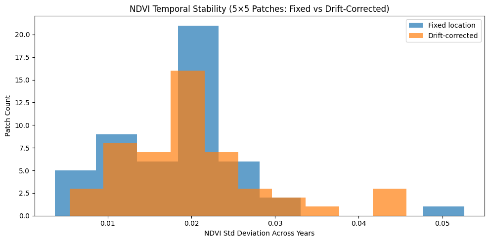
Interpretation:
NDVI temporal variance was slightly higher after drift correction, but the difference was not statistically significant. This suggests that 5×5 patches may already average out small shifts, providing inherent spatial robustness.
Pixel-Level (1×1)
| Metric | Fixed | Corrected |
|---|---|---|
| Mean NDVI std | 0.03982 | 0.02163 |
| T-statistic | 5.4654 | |
| P-value | 0.000002 |
Interpretation:
At the pixel level, drift correction substantially reduced NDVI variance over time. This indicates that raw pixel comparisons are highly sensitive to even minor misalignments, validating the need for patch-based or drift-corrected strategies in pixelwise classification.
Implications for Temporal Classification
This experiment confirms that spatial drift—though subtle—can meaningfully distort pixel-level change analysis. Without drift correction:
- Apparent transitions may be artifacts
- NDVI profiles become unstable
- Model errors can accumulate over time
In contrast, aggregating over 5×5 patches appears to mitigate these issues. For temporal studies involving land cover change, forest degradation, or regrowth detection, we recommend either:
- Drift correction per-pixel when doing fine-grained transition modeling, or
- Switching to patch-based classification frameworks.
Limitations and Next Steps
- Only 3 fixed reference points could be visually confirmed across years
- Drift was only modeled as linear (search radius ±3 pixels)
- NDVI was the only signal used for comparison (future versions may include full spectral MSE)
Class Transition Validation Under Drift Correction
To further quantify the impact of spatial drift, we evaluated how class transitions across years are affected by fixed vs. drift-corrected sampling. The goal was to check whether implausible transitions—e.g., BARE → DEAD or DEAD → LIVE—are more common when drift is not accounted for.
Motivation
Temporal classification relies not just on stable NDVI signals but also on reasonable class transitions. Certain transitions are biologically plausible (e.g., LIVE → DEAD → BARE), while others are not expected without long timescales or special conditions (e.g., BARE → LIVE over 2 years).
Spatial drift can artificially introduce these implausible sequences. This section evaluates whether correcting for drift reduces the frequency of such transitions across the entire buffer.
Hypothesis
If drift correction improves temporal alignment, then:
- The proportion of implausible transitions should decrease
- Heatmaps of transition probabilities should show more stability or logical progression
- This effect should be statistically significant
Method
For each pixel in the valid interior region of the buffer:
- Extract Class Predictions from 2014, 2016, and 2018
- Construct Fixed Sequences: row/col is held constant
- Construct Drift-Corrected Sequences: find the closest RGB patch match in the next year using 5×5 RGB context
- Count transitions of form: (class_t → class_t+1) for each consecutive year pair
- Tabulate transition matrices for both fixed and corrected cases
- Highlight implausible transitions, defined as:
- DEAD → LIVE
- BARE → DEAD
- BARE → LIVE
- Plot
- Heatmaps of transition probabilities
- Bar plots of total implausible transition percentages
Results
Heatmap: 2014 → 2016 Transitions
Heatmap: 2016 → 2018 Transitions
Bar Chart: Implausible Transition Rates
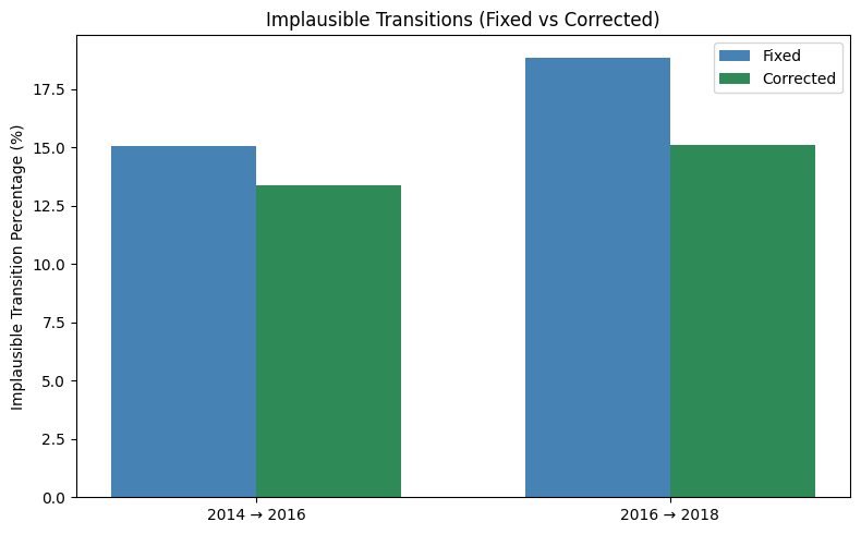
| Transition Period | Fixed (%) | Corrected (%) |
|---|---|---|
| 2014 → 2016 | 15.5% | 13.4% |
| 2016 → 2018 | 19.8% | 14.4% |
Statistical Test (Chi²):
- χ² Statistic: 144.07
- P-value: < 0.000001
→ Statistically significant improvement in plausibility after drift correction
Interpretation
- Heatmaps show that drift correction increases class stability, particularly for BARE and DEAD categories.
- The frequency of implausible transitions drops significantly when drift is corrected.
- Statistical testing confirms that this reduction is unlikely to be due to chance.
Final Takeaways
- Pixel-level NDVI analysis is highly sensitive to spatial drift
- Drift correction reduces implausible transitions and enhances temporal stability
- Patch-level aggregation is somewhat resilient to drift but less interpretable
- This two-pronged analysis—NDVI time-series + transition plausibility—offers a comprehensive method for diagnosing and mitigating drift in remote sensing studies