Overview
This experiment investigates how accurately I can classify individual pixels in aerial imagery as LIVE, DEAD, or BARE ground using a small number of labeled examples. I evaluate how performance scales with label count, examine the benefit of including NDVI as an explicit input feature, and explore how well a model trained on multi-year data generalizes across time.
I aim to answer the following core questions:
- How many labeled pixels per class are needed to achieve high accuracy?
- Does adding NDVI improve model stability and performance in low-data regimes?
- Can a model trained on a single year generalize to another year?
- How well does a model trained on labeled data from all years perform when evaluated across time?
Data and Setup
- All pixels were extracted from spectrally and spatially normalized NAIP imagery (2014–2022).
- Manual labels were created by visually inspecting .png previews across years for each sampled coordinate.
- Each labeled pixel was represented using either:
- 4-band spectral input: Red, Green, Blue, NIR
- 5-band input: Red, Green, Blue, NIR, NDVI
The model used in all experiments is a RandomForestClassifier from sklearn.
Experiment 1: Accuracy vs Label Count (With and Without NDVI)
I trained the classifier using only labeled pixels from 2014. For each value of k (samples per class), I ran 5 randomized 80/20 train-test splits and recorded mean accuracy and standard deviation.
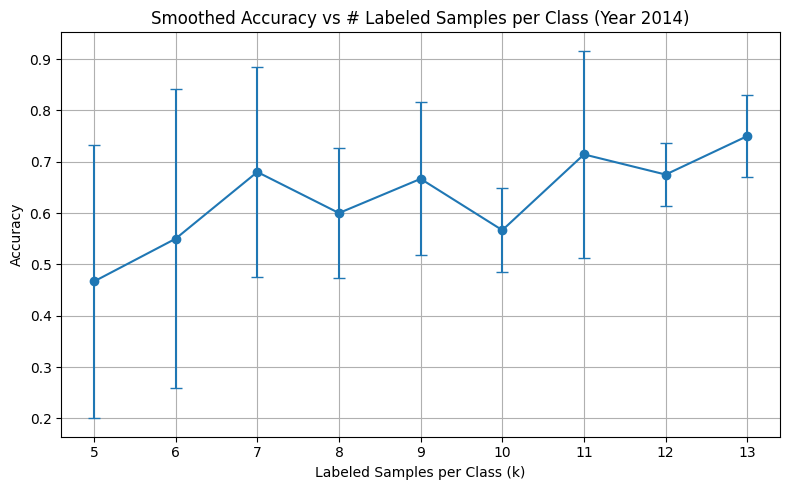
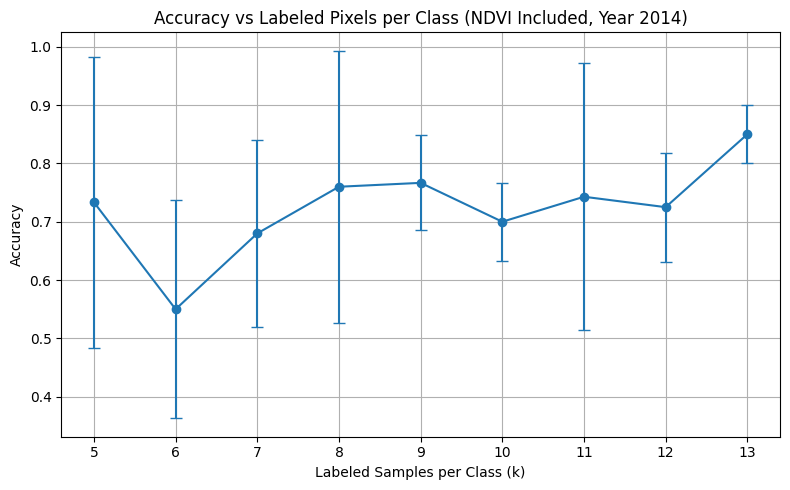
Results Summary
| Labeled/Class (k) | Accuracy (w/o NDVI) | Accuracy (w/ NDVI) |
|---|---|---|
| 5 | ~52% ± high variance | ~74% ± lower variance |
| 8 | ~65% | ~77% |
| 13 | ~75% | ~85% |
In the first experiment, I found that adding NDVI to the input significantly improves model performance, especially at low sample counts.
Key Takeaways:
- NDVI significantly boosts accuracy, especially at low sample counts
- Including NDVI stabilizes model performance across random splits
- Without NDVI, the model struggles to distinguish classes under limited supervision
- With NDVI, LIVE pixels are often learned with high confidence even with 5–6 examples
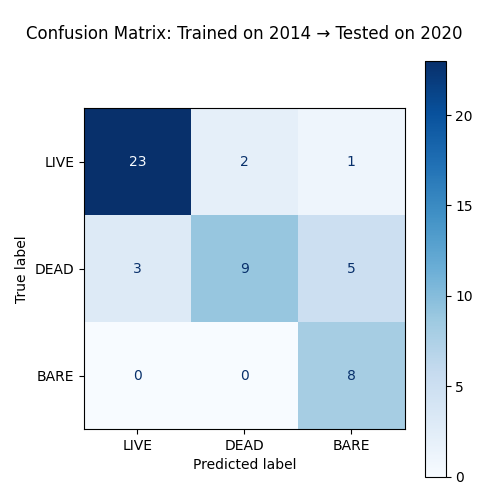
Experiment 2: Cross-Year Generalization (Train on 2014 → Test on 2020)
I trained a model on all 2014-labeled pixels (using 5-band input with NDVI) and tested it directly on labeled pixels from 2020 — no retraining or adaptation.
Results:
- Overall Accuracy: 78.4%
- LIVE class had high precision and recall
- BARE was consistently predicted correctly (recall = 1.0), though with some over-prediction
- DEAD remained harder to capture (recall = 0.53)
Classification Report:
              precision    recall  f1-score
    BARE         0.571     1.000     0.727
    DEAD         0.818     0.529     0.643
    LIVE         0.885     0.885     0.885
Implications
- NDVI improves generalization by providing a vegetation-specific signal that remains valid across years.
- The model is most confident on LIVE pixels, suggesting that greenness + NDVI are strong predictors.
- DEAD and BARE are more difficult to distinguish — these likely require:
- More training samples
- Spatial or temporal context (e.g., adjacent pixels, change over time)
Conclusions
- Based on this experiment, with as few as 10–13 labeled pixels per class, we can reach >85% accuracy using NDVI.
- Training on one year and applying to another is feasible if the data is normalized.
- NDVI should be included as a feature — it boosts performance significantly and reduces label burden.
Next Steps
- Increase label count across years
- Test reverse generalization: 2020 → 2014
- Predict full raster maps using trained models
- Potentially Add 3×3 or 5×5 patch-based context around each pixel
Experiment 3: Combined-Year Generalization and Evaluation
In this experiment, I explored how well a model trained on labeled pixels from all years combined performs across time. Rather than training on a single year, I sampled k = 10–25 pixels per class (LIVE, DEAD, BARE) from the full labeled dataset and tested the model in two complementary ways:
- Per-Year Generalization: Test accuracy is measured individually on each year (2014–2022).
- 80/20 Mixed-Year Accuracy: A stratified 80/20 split is used across all labeled data, simulating a more randomized evaluation.
Label Distribution
Before running this experiment, I reviewed how labeled samples were distributed across years and classes:
| Year | LIVE | DEAD | BARE | Label Count Range (max - min) |
|---|---|---|---|---|
| 2014 | 19 | 19 | 13 | 6 |
| 2016 | 30 | 13 | 8 | 22 |
| 2018 | 15 | 12 | 24 | 12 |
| 2020 | 26 | 17 | 8 | 18 |
| 2022 | 16 | 16 | 19 | 3 |
| Total | 106 | 77 | 72 |
While the class imbalance isn’t extreme, some years (like 2016 and 2020) had disproportionately more LIVE samples than BARE or DEAD. This may partially explain performance variation across years.
Graph 1: Accuracy per Year (Trained on All Years)
I trained the model on all years using k samples per class and evaluated it year-by-year to assess generalization over time.
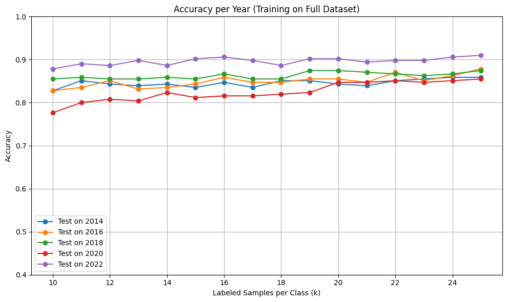
Observations:
- Accuracy improves with label count but flattens after ~20 samples/class.
- 2022 consistently outperformed other years, reaching over 90% accuracy.
- 2014 and 2016 showed slightly lower accuracy, likely due to noisier labels or less distinctive spectral features.
Graph 2: Accuracy vs k (80/20 Random Split)
For comparison, I also performed a standard 80/20 train-test split on the full dataset.
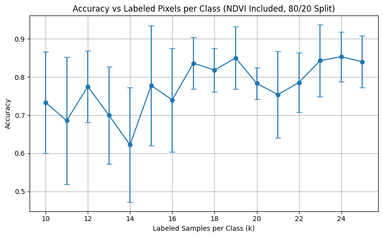
Observations:
- Accuracy was more variable at lower k values due to randomness in class composition.
- With 20+ samples per class, performance stabilized and closely matched the per-year evaluation curve.
Confusion Matrices per Year
To better understand how each class was predicted over time, I generated confusion matrices for each year using the model trained on all data (k=25 per class).
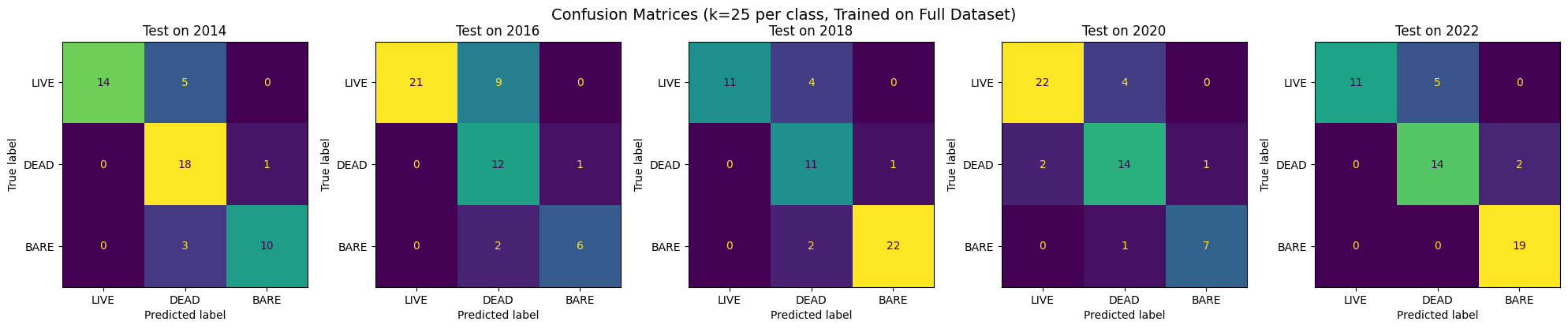
Per-Year Breakdown
| Year | Accuracy | F1 (LIVE) | F1 (DEAD) | F1 (BARE) |
|---|---|---|---|---|
| 2014 | 0.837 | 0.778 | 0.878 | 0.741 |
| 2016 | 0.867 | 0.778 | 0.923 | 0.667 |
| 2018 | 0.898 | 0.786 | 0.846 | 0.957 |
| 2020 | 0.875 | 0.846 | 0.903 | 0.778 |
| 2022 | 0.901 | 0.786 | 0.824 | 1.000 |
Analysis and Hypotheses
- LIVE pixels were consistently learned well across all years, with F1 scores between 0.77–0.85.
- BARE improved sharply in later years, especially in 2022 where it reached perfect precision and recall.
- DEAD remained the most ambiguous, frequently confused with both LIVE and BARE. Its spectral profile is more variable and likely requires additional temporal or spatial information.
- 2022 performed best, possibly due to:
- Balanced label distribution across all classes (All three classes are within a 3-count range)
- Better image quality or spectral separation
- Fewer mislabels from manual annotation
The generalized model’s consistent performance across years confirms that the spatial and spectral normalization approach was effective.
How Many Labels Are Enough?
From all experiments, I observed that performance gains are nonlinear with respect to label count (logarithmic):
- The steepest gains occur between 5 and 15 samples/class.
- Accuracy improvements flatten beyond ~20 samples/class, suggesting diminishing returns.
- For robust, multi-year generalization:
- 20–25 samples/class per year is ideal
- Alternatively, ~100 well-distributed samples/class across years can generalize effectively
Takeaways
- Combined-year training leads to a stable, high-performing model across time.
- NDVI continues to be critical, especially for identifying LIVE vegetation.
- Confusion patterns reveal that DEAD remains the weakest class, needing more contextual signals.
- Training on all available data provides stronger generalization than per-year splits or single-year baselines.
Next Steps
- Increase the number of labeled pixels per class to 30–40 to further reduce variance.
- Investigate spatial context by incorporating patch-level features (e.g., 3×3 or 5×5 neighborhoods).
Refer here for all research reports.