Drift Configuration Evaluation and Transition Matrix Optimization

Overview

Building on our previous work analyzing spatial drift in NAIP imagery, we now shift focus to discovering globally optimal drift configurations. Specifically, we aim to:

Evaluate all 625 possible drift configurations (0–4 pixel shifts in row and column) between two years.
Score each configuration using biologically inspired heuristics.
Visualize and compare transition matrices from fixed vs. drift-corrected rasters.
Statistically validate improvements in NDVI temporal consistency and transition plausibility.

This report also introduces two scoring mechanisms to distill each 3×3 transition matrix into a single numeric value:

Simple Score: A linear weighting that rewards identity transitions and penalizes implausible ones.
Composite Score: A multi-factored function accounting for ecological decay patterns, entropy (stability), and biologically implausible reversals.

Why 625 Drift Configurations?

NAIP imagery has a maximum documented spatial error of ±4 meters, or 4 pixels (1m resolution) in either direction. For each pixel in year 1, we test all combinations of potential displacements for both the reference (year 1) and the target (year 2) images:

Total drift combinations = 5 (row1) × 5 (col1) × 5 (row2) × 5 (col2) = 625

For each configuration, we:

Shift the raster accordingly.
Compute a full 3×3 transition matrix.
Apply the scoring functions described below.

Scoring Transition Matrices

Simple Score

SCORE = +1 × identity transitions (LIVE→LIVE, DEAD→DEAD, BARE→BARE)
       - 3 × implausible transitions (e.g., BARE→LIVE, DEAD→LIVE, BARE→DEAD)
       - 2 × LIVE→BARE, DEAD→BARE

This score linearly rewards stability and penalizes biologically suspect changes. Fast to compute, it provides an interpretable surface over the 625 space.

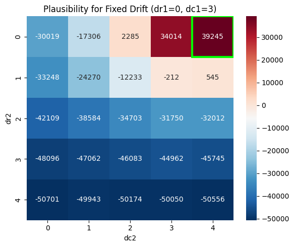
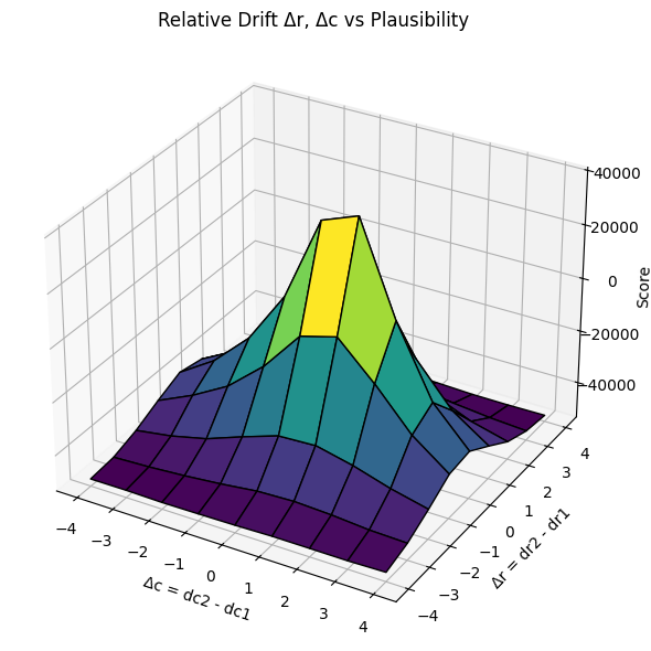
We visualized this in 2D heatmaps (fixed dr1, dc1) and a 3D surface showing plausibility as a function of relative drift ∆r, ∆c.

Figure 1 – Heatmap of Plausibility (Simple Score) Across Fixed Drift Combinations

Figure 2 – 3D Surface Plot of Drift ∆r, ∆c vs Score

Composite Score

The composite score integrates:

Decay Reward: Encourages LIVE → DEAD → BARE progression
Implausibility Penalty: Penalizes unnatural reversals (e.g., BARE → DEAD)
Entropy Penalty: Penalizes instability in row-wise transition distributions

SCORE = -Entropy + Decay Reward - Implausible Penalty

This metric encodes more biological realism and rewards transitions that align with ecological degradation.

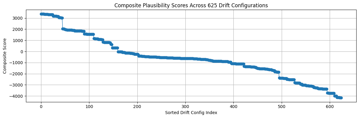
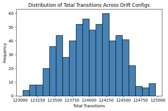
We plotted this across all 625 configurations and observed a long-tailed unimodal curve:

Figure 3 – Composite Score Distribution Over Drift Space

Comparing Best Drift Configs

We selected the top-scoring drift configurations under both schemes:

Simple Score: (0, 3, 0, 4)
Composite Score: (1, 3, 1, 1)

Below are the resulting transition matrices compared to the baseline (no drift):

Figure 4 – Simple Drift vs No Drift (Transition Matrix %)

Figure 5 – Composite Drift vs No Drift (Transition Matrix %)

Figure 6 – Simple vs Composite Drift (Transition Matrix %)

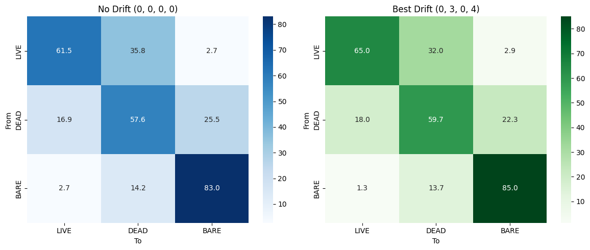
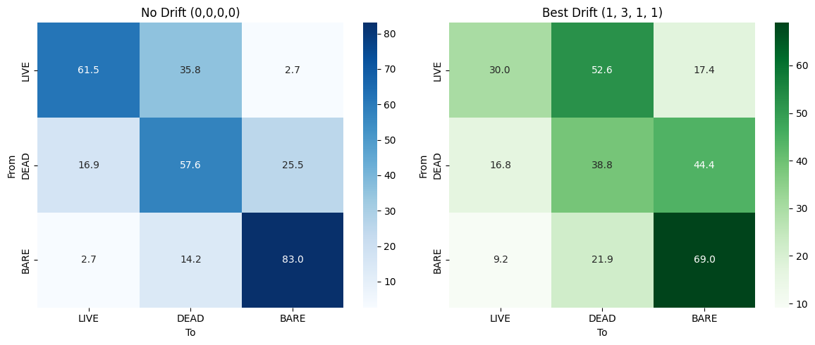
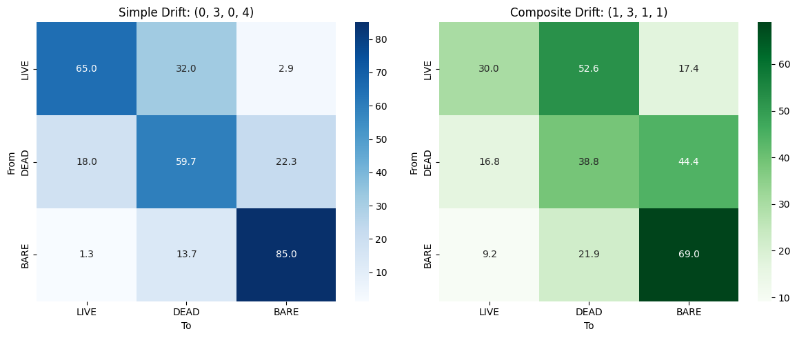
Observation

Simple drift yielded cleaner BARE → BARE diagonals and minimized reversal transitions
Composite score slightly favored plausible but diverse transitions with less focus on strict diagonal preservation

Note on Edge Effects and Pixel Exclusion

When applying spatial drift configurations (e.g., shifting pixels up to 4 rows/columns in each direction), some border regions in the raster fall outside the valid image bounds. To ensure consistency and prevent out-of-bounds indexing errors, these edge pixels were excluded from all transition and NDVI calculations.
As a result, the total number of pixels used in each drift configuration may vary slightly depending on how much drift was applied, especially in diagonally extreme configurations. These excluded pixels do not affect the comparative plausibility scoring, as the variation is negligible (<3% of total pixels), and only valid overlapping regions were considered in all evaluations.

Validating NDVI Temporal Stability

To evaluate temporal alignment, we computed pixelwise NDVI standard deviation across 5 years (2014–2022) for all interior pixels:

Fixed Coordinates: Use same pixel (r, c) each year
Drift-Corrected: Apply optimal drift (from 2014 and 2016 only) then use fixed (r, c) for future years

Result:

Metric	Fixed	Drift-Corrected
Mean NDVI Std Deviation	0.04544	0.05093
Paired t-test p-value	< 0.000001	(statistically significant)

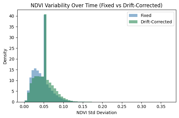
While the mean NDVI variability increased slightly under drift correction, the test remains a useful lens for validating long-term alignment.

Observing Score Differences

We analyzed the Spearman Rank Correlation between both scoring systems:

ρ = -0.2253, p < 0.000001 → Significant negative correlation

This suggests the scoring systems are not directly aligned, and each captures different facets of temporal plausibility

Final Takeaways

Optimal drift varies depending on scoring design and ecological intent
Simple scoring performs surprisingly well for suppressing implausible transitions
Composite scoring emphasizes ecological progression and entropy
NDVI-based variance is slightly worse under drift correction, but this may reflect better alignment with shifting canopies or shadows
This pipeline generalizes across time ranges and can be applied to all pairwise year transitions

Next Steps

Apply the same analysis for 2016 → 2018, 2018 → 2020, 2020 → 2022
Test alternate scoring functions (e.g., chi-squared divergence from expected decay)
Integrate the best drift config into training/validation for improved pixel classification
Track class-specific drift stability (e.g., BARE pixels across years)
Eventually aim for full spatiotemporal drift-corrected land cover analysis

Refer here for all research reports.